
Application of computer vision on laboratory sandbox investigations
GitHub repository link
Table of contents
Citing this work
This project is part of the Saline Intrusion in Coastal Aquifers (SALINA) research project.
This work was originally published under the title: Optimizing Laboratory Investigations of Saline Intrusion by Incorporating Machine Learning Techniques in the Water MDPI journal.
Project overview
Deriving saltwater concentrations from the values of light intensity is a long-established image processing practice in laboratory scale investigations of saline intrusion. The current repository presents a novel methodology that employs the predictive ability of machine learning algorithms in order to determine saltwater concentration fields. The proposed approach consists of three distinct parts, image pre-processing, ground profile classification (bead structure recognition) and saltwater field generation (regression). It minimizes the need for aquifer-specific calibrations, significantly shortening the experimental procedure by up to 50% of the time required.
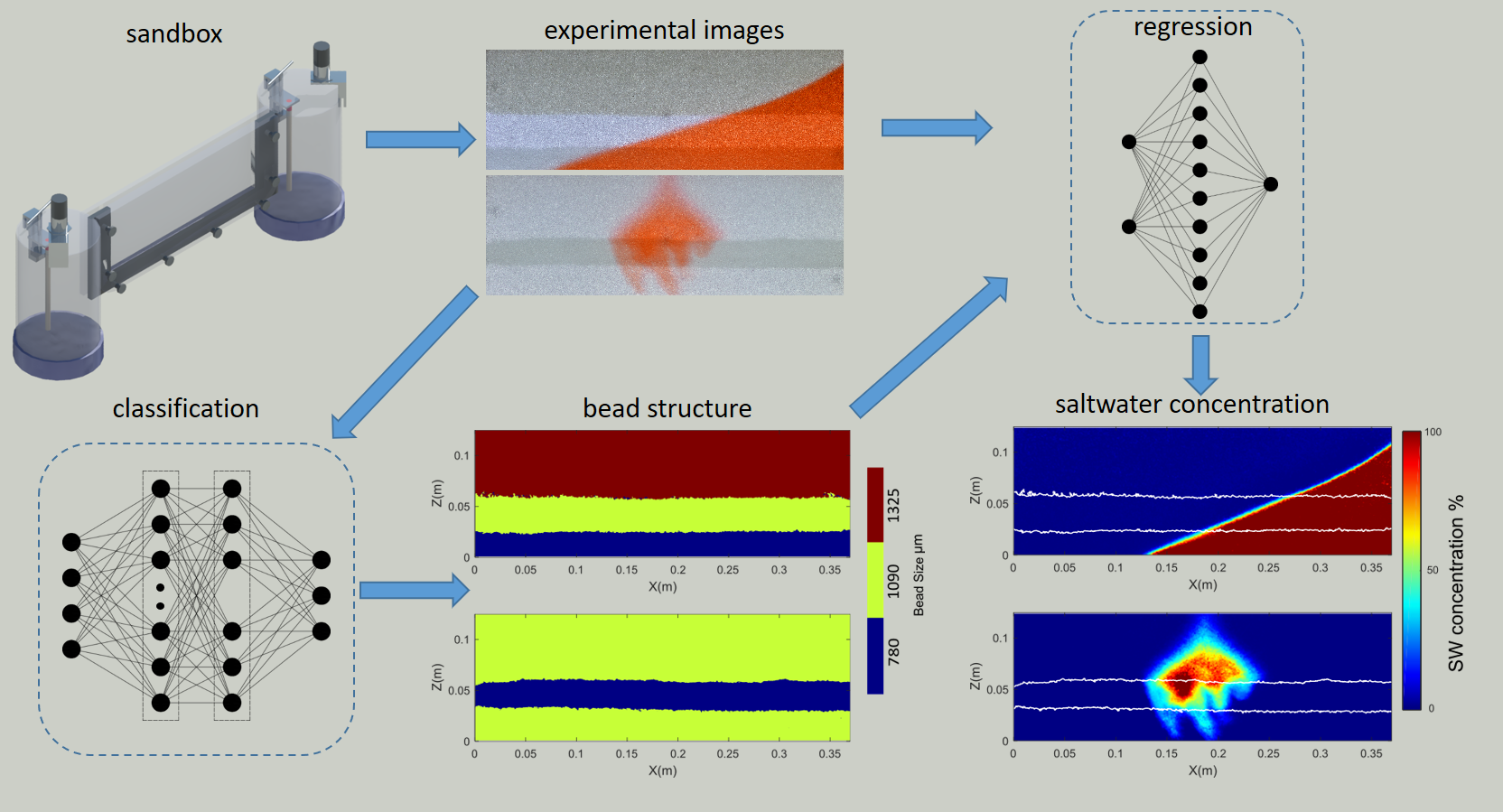 A graphical outline of the investigation
The methodology introduced in this investigation comprises three sections. The first part involves experimental image pre-processing via both established and novel procedures. The second part treats the task of recognizing aquifer heterogeneity as a multinomial pixel wise classification problem. Lastly the third section derives the saltwater concentration fields via regression analysis on the values of light intensity (LI) and the corresponding bead sizes.
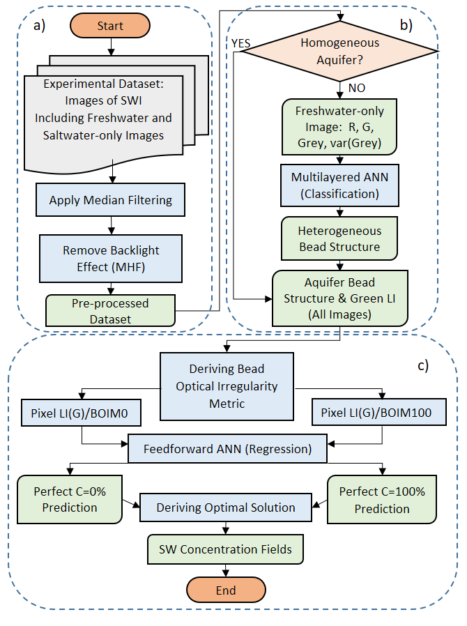 Flowchart of the proposed methodology depicting its three distinct parts a) image pre-processing, b) bead structure recognition (classification) and c) saltwater field generation (regression)
Data description
A thin sandbox setup was used to recreate the experimental data utilized in this project. The coastal aquifers were approximated by filling the central chamber with clear glass beads of three predetermined diameters (780 μm, 1090 μm, 1325 μm). In most test cases the reservoir on the left was filled with fresh water, while the one on the right contained dyed (red) saltwater. Two fine mesh acrylic screens were used to retain the beads in the main part of the apparatus while still permitting water circulation between the two tanks and the viewing chamber. Adjustable overflow outlets controlled the water level in the two side chambers and incremental changes in water level were achieved via the use of two ultrasonic sensors. The measurements took place in a totally dark room.
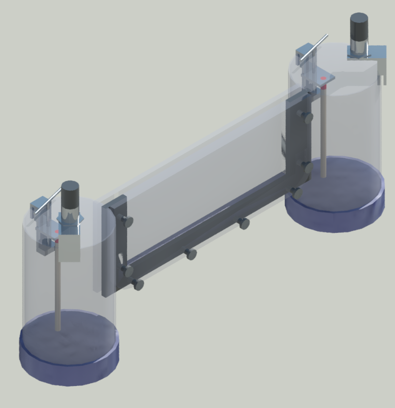 3-d depiction of the experimental sandbox setup
During the classification analysis, freshwater-only photos of the experimental aquifers were used. Homogeneous aquifers served as training and testing data, while stratified ones were strictly used for testing.
The regression anlysis part involved two categories of data, calibration and test images. Calibration images were created by filling homogeneous aquifers (one for every utlized bead size) with saltwater - freshwater solutions of predetermined concentrations, where SW = 0 %, 5 %, 10 %, 20 %, 30%, 50 %, 70 %, 100 %. Test images were created by generating either a saltwater wedge or a saline plume in stratified coastal aquifers.
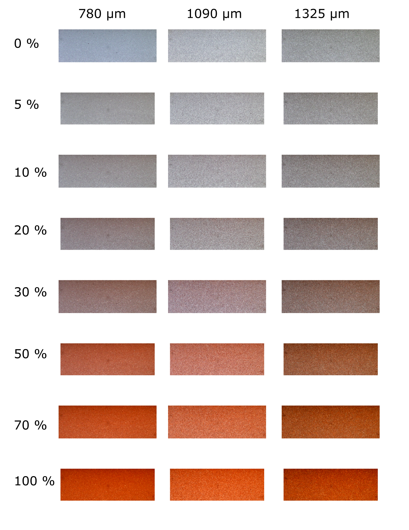 The 24 calibration images utilized in the investigation
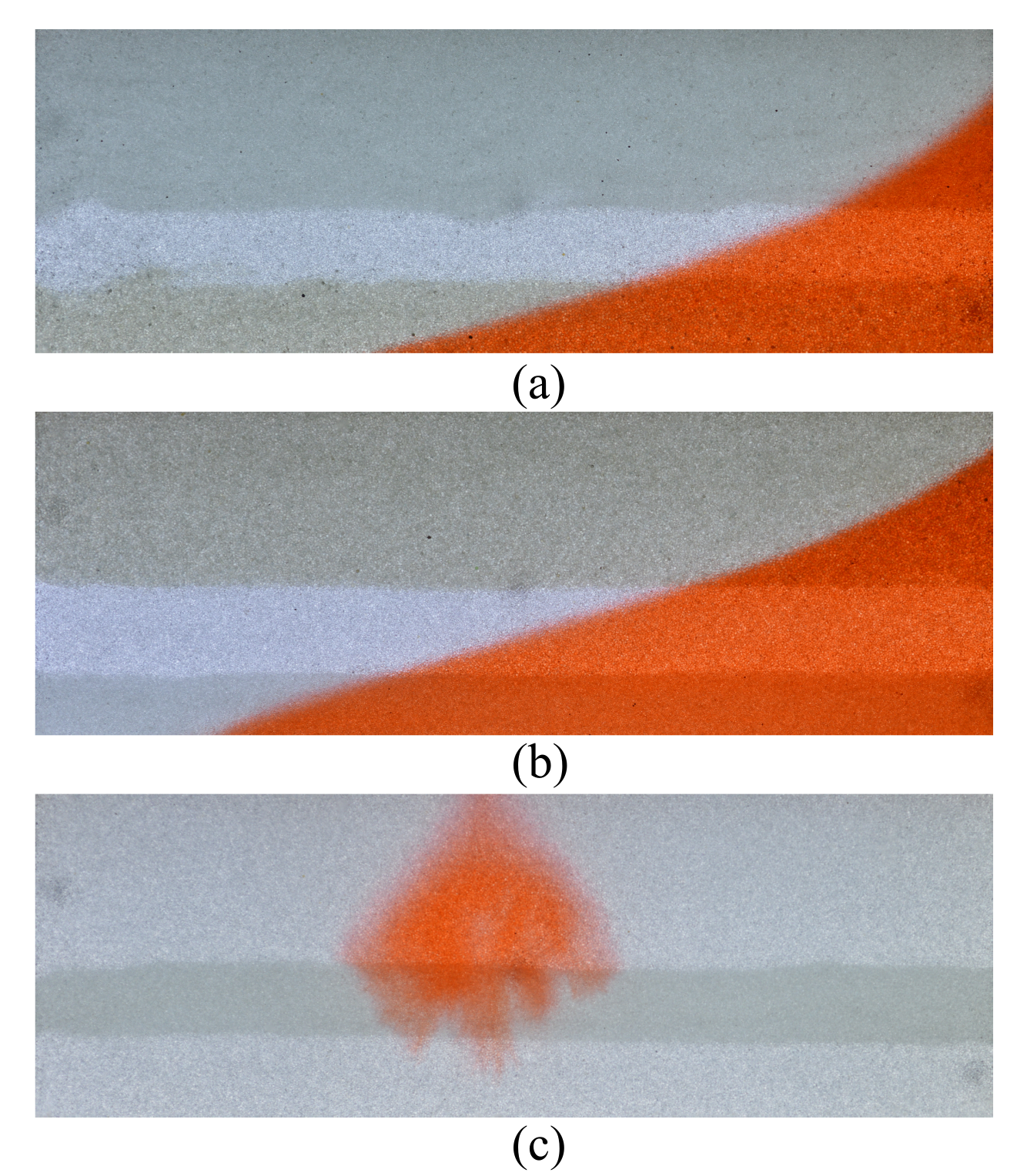 Three test images demonstrating different types of saline intrusion in stratified aquifers
Three homogeneous aquifers served as the training datasets for all the machine learning algorithms. The remaining aquifers were utilized for quantifying the models’ generalization ability. It was established that one homogeneous aquifer per bead size used, generated sufficient data for the successful implementation of the method. After the training of the neural learners was complete, saltwater concentration fields could be successfully generated with no further calibration effort for any number of new homogeneous or heterogeneous aquifers.
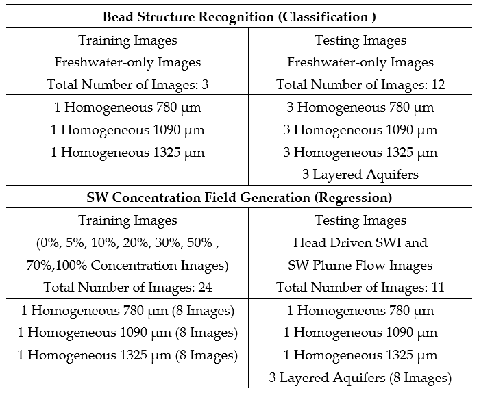 Experimental aquifer images used as training and testing datasets by the classification and regression machine learning algorithms
Image pre-processing
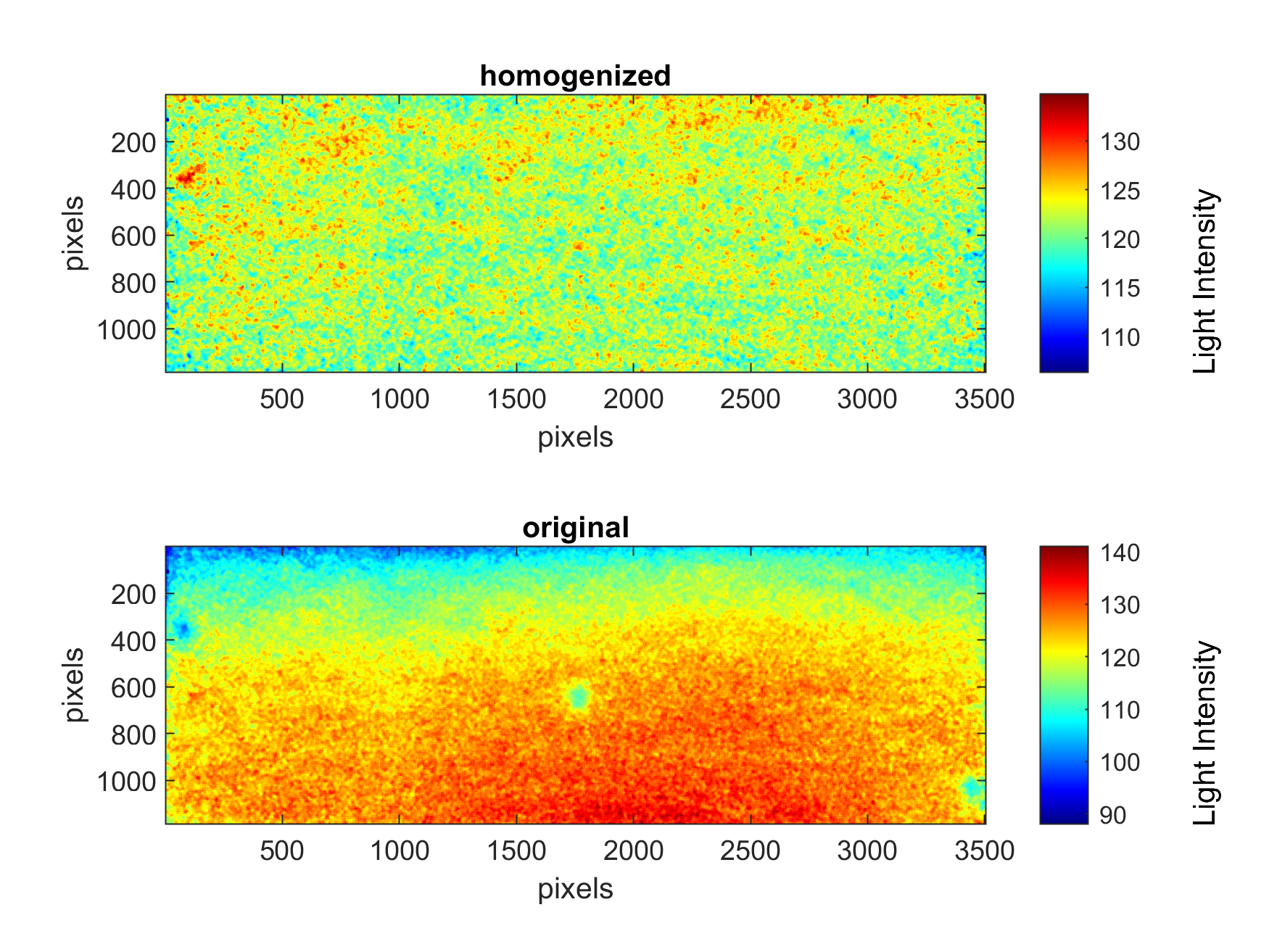
Data pre-processing significantly affects the generalization performance of supervised machine learning algorithms. Τhe images of homogeneous aquifers were characterized by significant irregularity in the distribution of light intensity values. This can be attributed to two distinct factors: the different optical attributes of each specific glass bead and the lighting conditions. While the first cause creates a random variation in the observed LI values, the second is responsible for a distinct distribution, where the images appeared lighter in the centre of the sandbox.
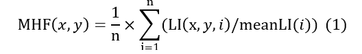
This lighting pattern was efficiently filtered out by developing the Mean Homogenization Factor (MHF) presented in this equation:
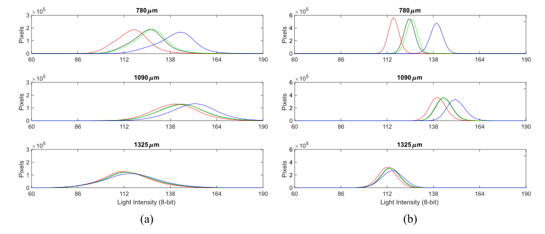 Light intensity distribution of the a) original and b) homogenized training images
 Impact of Mean Homogenization Factor on a single homogeneous aquifer photo
The application of MHF contributed to a significant improvement in the training and generalization performance of the machine learning algorithms tested in the next section.
Folder material description
Scripts: MeanHomoFactorCalculator.m
Datasets: subset1.mat, subset2.mat, subset3.mat, subset4.mat (containg 12 freshwater-only images of homogenoeus aquifers)
Classification
This part gives the user the ability to recognize the size of individual beads and thereby any given heterogeneous structure through a soft-computing method based on supervised machine learning. The technique enables the automatic recognition of more complex, including totally random, experimental aquifers, while minimizing the time needed for recreating each one of them. This part of the investigation is based on images of the 15 aquifers taken prior to saltwater intrusion. The pixels of three homogeneous aquifers served as the training subset. The remaining twelve images were used to evaluate the effectiveness of the method. The training subset was deliberately kept as small as possible, in order to ensure the easy implementation of the approach.
a) Classification training
Folder material description
Scripts: ClassificationTrainingData.m (prepares data for neural training),
ANNClassifiationGenerator.m (trains on parallel a deep classification ANN)
Data: subset4.mat (used as the training dataset, containing 3 freshater-only aquifer images, one for every utilized bead size)
Necessary variables: MeanHomofactorRGB.mat derived from the execution of MeanHomoFactorCalculator.m
b) Classification prediction
The classification prediction data generated by ClassificationData.m were subsequently fed into a trainned deep neural network using ANNPrediction.m. The final result was as follows:
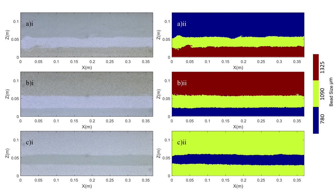 Heterogeneous aquifers (i) and the (ii) bead structure generated by a multi-layered Artificial Neural Network (ANN)
b) Classification prediction post processing using ANNPredictionProbability.m
An alternative prediction algorithm was proposed to further improve the predicted heterogeneous structure. When the softmax activation function is used on the output layer of neural networks, the likelihood of the observations belonging to each predetermined class is returned as a probability vector. As expected, most of the misclassification occurrences are correlated with predictions of relatively high uncertainty. A post-processing algorithm was created to filter out the misclassifications using the probabilistic nature of neural network predictions. Initially, pixels whose size was identified with a probability lower than 99.9% were determined (Fig. b). Next, a subroutine investigated the existence of dominant bead size around these pixels in a neighborhood of varying dimensions. If a dominant bead diameter was identified, its value was assigned to the pixels in question. This procedure filtered out the highest percentage of unsuccessfully predicted bead sizes (Fig. c). Subsequently, a similar search subroutine was applied in the whole image to filter out any pixels that were initially misclassified with a probability higher than 99.9%. Special precaution was taken against altering the interface between different bead layers. The final bead structure prediction (Fig. d) constitutes a near perfect representation of the bead strata both in this and the remaining heterogeneous aquifers. This post processing method is fully automated. User interference is limited to determining the minimum size of heterogeneous structure present in the aquifer.
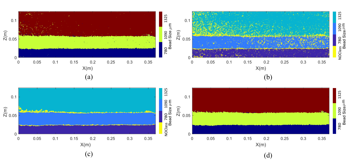
The four prediction steps executed in ANNPredictionProbability.m
Folder material description
Scripts: ClassificationData.m (prepares data for testing),
ANNPrediction.m (executes the neural prediction),
ANNPredictionProbability.m (executes the neural prediction while further post-processing it to get optimum results)
Data: ANNclassification.mat (pre-trained deep classificstion neural network),
testdataset.mat (3 stratified test aquifers)
Necessary variables: MeanHomofactorRGB.mat derived from the execution of MeanHomoFactorCalculator.m
Regression
The image processing methods that have been presented up to now were based on the same principle. A number of calibration images were acquired for each aquifer, these data were used to formulate a relationship between LI values and SW concentrations via regression analysis. While relatively accurate, these techniques were disadvantaged by the need to acquire new calibration images for every investigated aquifer, making them slow and labour intensive. Eliminating this need by the use of machine learning, will represent a step change in the ability to run significant laboratory investigations.
a) Regression training
A traditional MLT approach would feed the raw data from the eight calibration images (with saltwater concentrations of 0%, 5%, 10%, 20%, 30%, 50%, 70%, and 100%), of one homogeneous aquifer for each utilized bead size, into a sufficiently strong learner that would automatically establish a relationship between LI and SW%. Nevertheless, it is well documented that experimental data of saltwater intrusion generated in sandbox setups are characterized by a high percentage of irregularity, mostly due to the deviating light absorbing attributes of the individual beads.
The nature of this type of data constitutes their straightforward use for neural training problematic. Instead of the actual images, a feedforward ANN with one 10-neuron hidden layer was trained on the mean values of monochromatic green LI for each specific aquifer using Levenberg–Marquardt as its training algorithm.
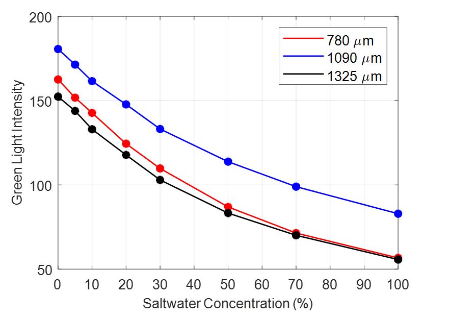 Average values of green light intensity of the three homogeneous aquifers for each corresponding calibration concentration
Folder material description
Scripts: RegressionTrainingData.m (prepares data for neural training),
ANNTrainingRegression.m (trains on parallel a regression ANN)
Data: Cal780G.mat, Cal1090G.mat, Cal1325G.mat (green (G) light intensity values for each one of the utilized bead sizes, each subset includes the 8 calibration concentration images)
b) Regression prediction
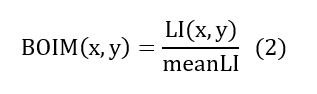
In order to minimize the impact of noisy data, caused by the presence of beads of varying colour tones, a quantification of the optical irregularities of the glass bead medium was essential. This procedure took place in the freshwater only images of the tested aquifers. To do so the LI values of each individual pixel were divided with the corresponding measured average LI value of its bead size. In doing so, a Bead Optical Irregularity Metric (BOIM) was derived characterising each specific bead of the investigated aquifers as shown in Equation 2, assigning higher and lower BOIM values to lighter and darker beads respectively.
By dividing the freshwater only image of any aquifer with its corresponding BOIM matrix, the mean LI values the feedforward ANN was trained upon are returned. When these values were fed on the neural network the 0 % SW concentration fields was perfectly recreated. The same procedure was repeated for saltwater-only images of the aquifers, deriving the BOIM corresponding to the 100% saltwater percentage. This leading to perfect prediction of the 100% SW concentration components of the testing images. Dividing the SWI test images with BOIM0 and BOIM100 creates two data subsets that, when fed to the neural network, generate a perfect prediction of the two main concentration regions.
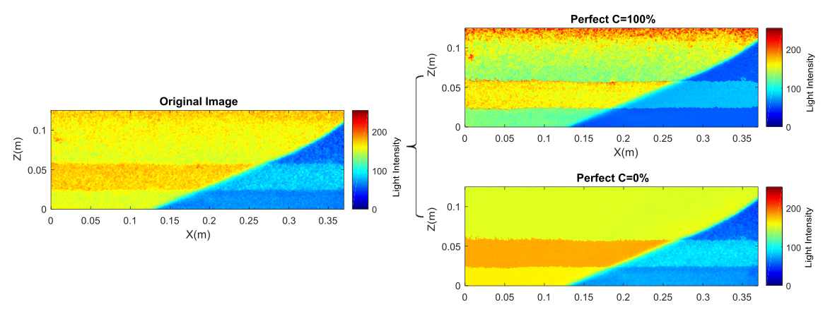 Effect of the implementation of BOIM0 and BOIM100 on a SWI image of the Layered2 aquifer
A crucial step towards the correct representation of the mixing zone on the salt-freshwater interface was the proper combination of values of the two, BOIM0 and BOIM100-modified, SW concentration fields. The next figure illustrates the mean squared error (MSE) generated by the ANN for the actual data of the homogeneous calibration images, expressing the difference between the calculated and the real SW%. For concentrations closer to 0%, the BOIM0-modified subsets generate less MSE. The same applies to the BOIM100-modified figures for bigger SW concentrations.
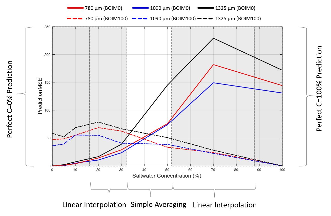 Mean squared error generated by the BOIM0 and BOIM100 modified subsets for the three homogeneous aquifers and the proposed optimum combination of the predictions
A prediction combination based on this error distribution was formulated. For extremely small or big saltwater concentrations only the BOIM0 (zone 1) and the BOIM100 (zone 5) predictions were taken into account. In between zones 1 and 5, three distinct zones were favoured, where either simple (zone 3) or weighted averaging (zones 2 and 4) between the two predictions took place.
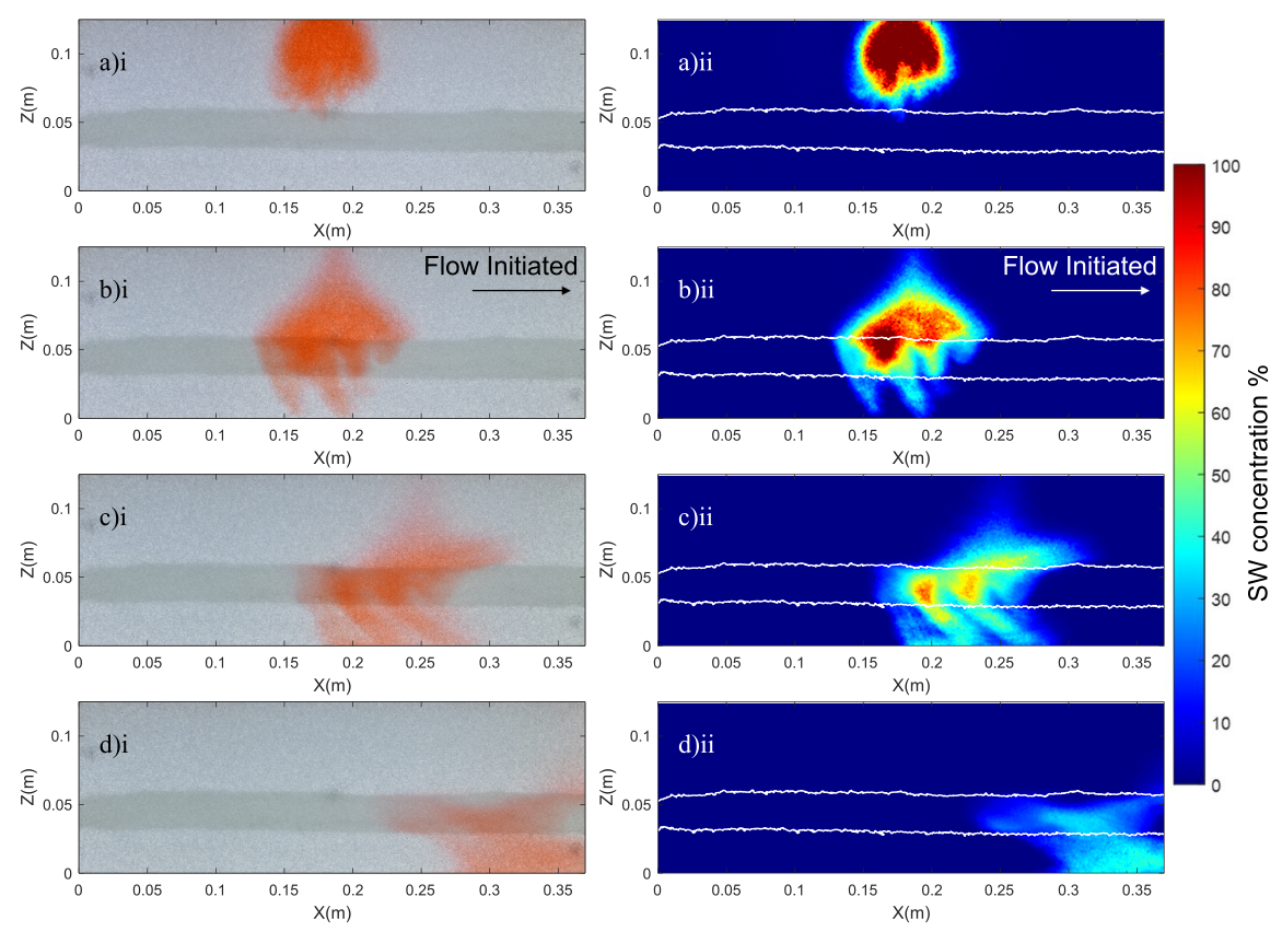 Experimental images (left) and saltwater concentration fields (right) generated by the proposed ML technique
Folder material description
Scripts: RegressionTestData.m (prepares data for testing),
ANNPredictionRegression.m (executes the neural prediction),
Data: ANNregression.mat (pre-trained regression neural network),
Str10907801090.mat (aquifer heterogenous structure derived from the classification analysis of the previous section),
Layered3SW0.mat, Layered3SW100.mat, Layered3Test1.mat (Green (G) light instensity values of saline intrusion test images in a heterogeneous aquifer)
Necessary variables: MeanHomofactorRGB.mat derived from the execution of MeanHomoFactorCalculator.m
c) Genetic algorithm optimization
This part determines the optimum combination between the Perfect C=0% and Predect C=100% predictions generated by the ANN in the previous section.
The calculation of the mean squared error was based on the 24 calibration images of the three homogeneous aquifers. The algorithm’s objective function included five variables, representing the width of each zone (x1, x2, x3, x4, x5). Since calibration concentrations were skewed towards 0%, using the total MSE generated for the aforementioned images as the algorithm’s objective function, would constitute an underestimation of the error in bigger concentrations. A weighted averaging of the MSE between every two consecutive calibration images was used instead for each one of the 3 aquifers:
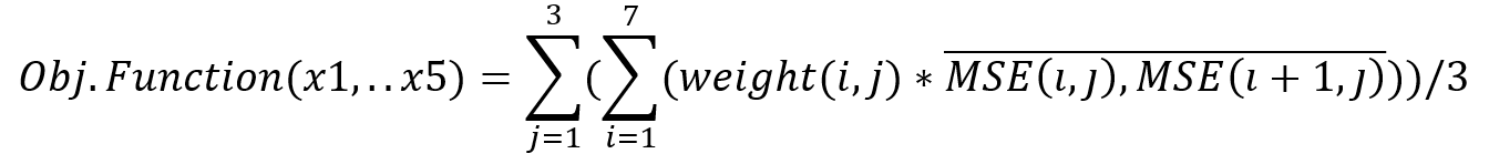
where j is the number of homogeneous aquifers (three) and i is the number of calibration concentrations (eight). An initial solution population of 500 was deemed sufficient, while the genetic procedures were implemented for 100 generations. The algorithm was executed for a total of eight times to derive the optimum solution.
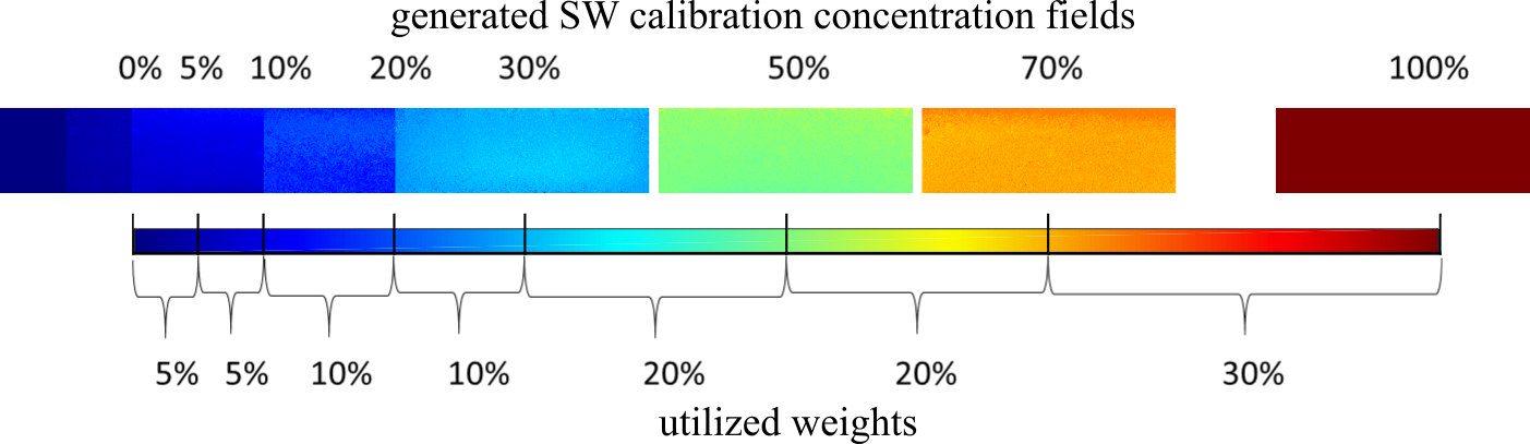 Calculation of weights for the weighted averaging of generated Mean Squared Error
Folder material description
Scripts: GeneticAlgorithmSWCombination.m (main script executing the genetic algorithm iotimization),
ObjectiveSWcombination.m (the objective function that was optimmized),
gaplotbestcustom.m (ploting function)
Data: PredictionC0.mat, PredictionC100.mat (ANN prediction results for the 24 calibration images,corresponding to 3 homogeneous aquifers),
RealSW.mat (the actual calibration concentration of the 24 images, used to evaluate the preformance of the neural prediction)